ARIMA vs. XGBoost vs. LightGBM: A Full Walk-Forward Comparison
Five FRED loan-delinquency series, an identical walk-forward backtest for every model, a data-leakage bug caught before any result was trusted, and a formal significance test on what’s left after the leak is fixed.
A classical ARIMA baseline was tested, honestly, against XGBoost and LightGBM on real quarterly loan-delinquency data: same walk-forward evaluation for every model, real significance testing, and no result trusted until it survived scrutiny. A leakage bug in the first ML implementation produced an implausibly good early result; once fixed, ARIMA won every comparison, and SHAP explains why.
- ARIMA beat XGBoost and LightGBM on all five FRED loan-delinquency series, walk-forward backtested with an identical evaluation protocol for every model.
- A real data-leakage bug was caught before any ML result was trusted: a boundary condition in the direct-horizon target construction let a handful of training rows see their own test-window answer. Fixed and covered by a regression test.
- ARIMA’s advantage is statistically significant in 27 of 40 series/model/horizon comparisons (Diebold-Mariano, Harvey-Leybourne-Newbold corrected), universal at the 1-quarter horizon and fading at longer horizons.
- SHAP interpretability shows why: in all 10 of 10 series/model combinations, the single most recent lag carries 47–59% of total feature importance: both approaches lean on essentially the same signal, and ARIMA simply expresses it more efficiently on ~140 rows than a tree ensemble can.
Five accounts, one evaluation rule for every model
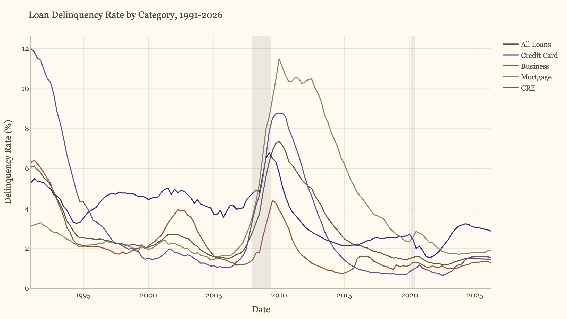
Data: FRED, quarterly, 1991-01-01 through 2026-04-01 (142 observations per series), truncated to that range at pull time.
- Series
- DRALACBS (All Loans), DRCCLACBS (Credit Card), DRBLACBS (Business), DRSFRMACBS (Mortgage), DRCRELEXFACBS (CRE)
- Backtest window
min_train_size = 80,h = 4quarters ahead, expanding window, refit every fold: 59 graded folds per series- Benchmarks
- Seasonal-naive (lag-4) and simple-naive (lag-1)
- Scoring metric
- MASE: mean absolute error of the model, divided by mean absolute error of the naive benchmark, averaged per fold
MASE = mean(|actual − predicted|) / mean(|naive benchmark error|)
Below 1.0 means the model beats the naive benchmark. Every model in this study (ARIMA, XGBoost, and LightGBM) is scored on the exact same 59 folds per series, so every number that follows is directly comparable across models.
Stationarity, autocorrelation, decomposition
ADF (H0: unit root) and KPSS (H0: stationary) were run on each raw series, at the conventional α = 0.05:
| Series | ADF p | KPSS p | Verdict |
|---|---|---|---|
| All Loans | 0.256 | 0.100 | Conflicting |
| Credit Card | 0.690 | 0.010 | Both: non-stationary |
| Business | 0.007 | 0.010 | Conflicting |
| Mortgage | 0.390 | 0.100 | Conflicting |
| CRE | 0.003 | 0.004 | Conflicting |
A conflicting ADF/KPSS verdict typically indicates trend-stationary behavior rather than test failure: real short-run mean reversion riding on top of longer, crisis-driven trend moves. ACF/PACF showed the classic AR signature (sharp PACF cutoff after lag 1–2, gradually decaying ACF) in every series, motivating AR(2) as the initial order guess for All Loans/Business/Credit Card/Mortgage and AR(1) for CRE. STL decomposition (period=4) confirmed trend dominates seasonality by an order of magnitude in every series, with both seasonal amplitude and residual variance expanding specifically during crisis windows, evidence of heteroscedasticity that motivated using conformal, error-history-based prediction intervals for the ML models rather than a fixed-variance assumption (see Prediction Intervals, below).
Full EDA write-up, all five ACF/PACF and STL plots: docs/phase1_eda.md in the project repository.
Per-series order search, diagnostics, backtest
Per series: a 5-candidate order grid built around the AR guess: (p,0,0), (p,1,0), (p,0,1), (p,1,1), (p+1,1,0), fit by maximum likelihood, lowest-AIC order selected, then walk-forward backtested.
| Series | Best order | Ljung-Box p (lag 4/8/12) | MASE vs. seasonal-naive | MASE vs. simple-naive |
|---|---|---|---|---|
| All Loans | (2,0,0) | 0.978 / 0.996 / 0.999 | 0.269 | 1.022 |
| Credit Card | (2,1,0) | 0.975 / 0.999 / 0.999 | 0.325 | 1.001 |
| Business | (2,1,0) | 0.989 / 0.999 / 1.000 | 0.236 | 0.866 |
| Mortgage | (2,1,0) | 0.986 / 0.977 / 0.991 | 0.348 | 1.148 |
| CRE | (1,1,0) | 0.994 / 1.000 / 1.000 | 0.135 | 0.524 |
All five pass Ljung-Box comfortably at every lag, no significant residual autocorrelation left unmodeled. One caveat worth stating plainly: by the conventional Burnham & Anderson rule of thumb (ΔAIC < 2 implies no decisive separation), four of the five winning orders are not decisively separated from their runner-up. CRE is the exception, and not on the top-two orders: it’s d=1 vs. d=0. ΔAIC of over 220, an unambiguous signal despite CRE’s formally ambiguous ADF/KPSS verdict above.
Feature construction and direct-horizon models
Univariate only: lags and rolling statistics of each target series itself, no exogenous variables, for the cleanest possible apples-to-apples comparison against ARIMA:
- Lags
[1, 2, 3, 4, 8]quarters: 1–4 covers the AR order Phase 2 already selected as best; 8 gives a 2-year lookback- Rolling features
- 4-quarter trailing mean and standard deviation
- Forecast strategy
- Direct, per-horizon: one model trained per forecast step (h=1..4), not recursive; no error compounding across the horizon
- Model scope
- Per-series (5 independent models) and one global model pooling all 5 series with a one-hot
series_idfeature - Hyperparameters
max_depth=3,learning_rate=0.05, subsampling, L2 regularization: shallow and regularized by design, given ~80–140 rows per fold
The bug: direct-horizon target leakage
target_h{h} = value.shift(-h) only produces NaN at the tail of the entire series, never at a fold boundary. The first implementation trained on every row in a fold’s training window, including the last h rows, whose targets land at positions i, i+1, …, i+h-1, inside that same fold’s own test window.
usable_train_idx = train_idx[train_idx + step_ahead ≤ train_idx[-1]]
Caught because an early Optuna tuning run produced an implausible result: one series’ outer-fold MASE dropped from a plausible 0.18 to 0.025 after only 5 trials. Verified directly (a fold’s last training row’s target position exceeded the fold’s own cutoff), fixed with the guard above, and pinned down with a dedicated regression test so it can’t silently reappear.
MASE vs. seasonal-naive, all five series
Pooling all five series into one global model (one-hot series_id) helped both ML models on 4 of 5 accounts over their own per-series version (more effective training rows), but did not close the gap to ARIMA on any account:
| Account | XGBoost (per-series) | XGBoost (global) | LightGBM (per-series) | LightGBM (global) |
|---|---|---|---|---|
| All Loans | 0.601 | 0.405 | 0.510 | 0.410 |
| Credit Card | 0.770 | 0.677 | 0.833 | 0.705 |
| Business | 0.660 | 0.646 | 0.643 | 0.651 |
| Mortgage | 1.663 | 0.935 | 1.490 | 1.081 |
| CRE | 0.537 | 0.377 | 0.515 | 0.394 |
Diebold-Mariano test: is ARIMA’s edge real?
The Diebold-Mariano test compares two models’ forecast-loss series and asks whether the difference is real or within sampling noise. With only ~59 folds per series (not thousands), the Harvey-Leybourne-Newbold small-sample correction was applied, using a Newey-West-style long-run variance with h-1 lags to account for the serial correlation h-step-ahead forecast errors carry.
DM = mean(d) / √(long-run-var(d) / T), dt = loss(e1,t) − loss(e2,t)
Run per series × model × horizon (40 comparisons, 59 folds each). ARIMA is significantly more accurate (p<0.05) in 27 of 40 comparisons, and directionally favored in all 40 of 40: the non-significant cells are “not proven at 5%,” never reversed.
Series-level pattern: Business (LightGBM) and Mortgage (XGBoost) go 4-for-4 significant; Credit Card loses significance cleanly at h=3/h=4 on both models; All Loans is the weakest of the five, with LightGBM losing significance starting at h=2.
Native ARIMA intervals vs. walk-forward conformal
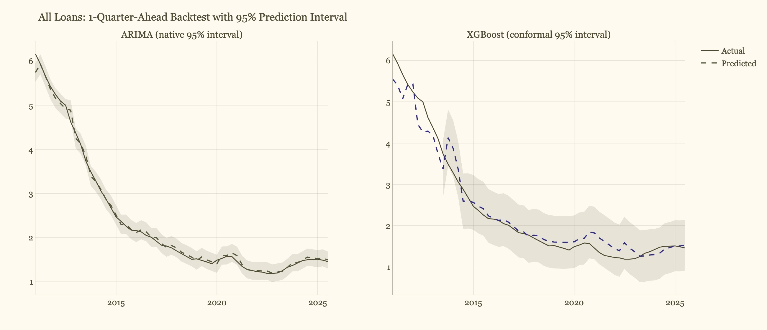
ARIMA gets calibrated intervals almost for free via get_forecast().conf_int(). Tree models don’t: a walk-forward-safe split-conformal method was used instead: the interval half-width for horizon h is the (1−α)-quantile of that horizon’s past absolute errors only (folds strictly before the current one), so there’s no leakage into the interval itself, on top of the point-forecast leakage guard above.
| ARIMA (native) | XGBoost (conformal) | LightGBM (conformal) | |
|---|---|---|---|
| Coverage of nominal 95% | 0.979–1.000 | 0.750–0.826 | 0.775–0.826 |
SHAP: what are the models actually looking at?
One final model per horizon, fit on all available history (there’s no future fold left to hold out for a model meant for actual deployment), explained with shap.TreeExplainer.
value_lag1’s share of total SHAP importance: the single most recent quarter, nothing else, at 47–59% of the entire decision, in all 10 of 10 series/model combinations.This is the mechanism behind the significance results above: ARIMA and the ML models converge on the same signal, but ARIMA writes it down directly in its coefficients while the tree ensembles spend a few hundred splits and ~80–140 training rows rediscovering roughly the same relationship.
Nested Optuna search: does tuning actually help here?
The fold sequence for each series was split by time order (not randomly) into the earliest ~70% (inner, 41 folds: Optuna searched here, 20 trials, minimizing mean backtest MAE) and the latest ~30% (outer, 18 folds, never touched by the search). Both fixed-default and tuned numbers below are evaluated on the same untouched outer folds.
| Account | Model | Fixed-default | Tuned | Helped? |
|---|---|---|---|---|
| All Loans | XGBoost | 0.623 | 0.622 | marginal |
| All Loans | LightGBM | 0.558 | 0.542 | yes |
| Credit Card | XGBoost | 0.719 | 0.757 | no |
| Credit Card | LightGBM | 0.843 | 0.764 | yes |
| Business | XGBoost | 0.311 | 0.382 | no |
| Business | LightGBM | 0.307 | 0.358 | no |
| Mortgage | XGBoost | 0.270 | 0.309 | no |
| Mortgage | LightGBM | 0.290 | 0.277 | yes |
| CRE | XGBoost | 0.390 | 0.412 | no |
| CRE | LightGBM | 0.398 | 0.450 | no |
Tuning helped in only 4 of 10 combinations, and made the outer-fold result worse in 6 of 10, consistent with the small-N overfitting risk that motivated trying fixed defaults first.
Model complexity has to match data size
For this problem (univariate, ~140-quarter macro series, direct-horizon forecasting), classical ARIMA is the stronger model, significantly so on the majority of series/horizon combinations. Global pooling and hyperparameter tuning both help the ML side somewhat but don’t close the gap.
With only ~140 observations per account, a 3-parameter model can be estimated reliably; a model built from hundreds of tree splits needs more data than that to find structure ARIMA doesn’t already capture. SHAP confirms it isn’t a training or tuning problem: both approaches are extracting the same signal, one just does it more efficiently at this sample size. The one lever that could plausibly change this result is genuinely new information (an exogenous macro regressor ARIMA never had access to either), not further feature engineering on the same short series.
Full code, tests (23 passing), and reproducible pipeline scripts in the linked repository, including the golden-snapshot regression suite, the leakage-guard regression test, and every script used to produce the numbers above. View on GitHub.